Welcome to QM-Thermodynamics’s documentation!
Ab initio calculation of an equation of state and thermodynamics of minerals
Thermodynamic properties, equation of state (3th or 4th-order Birch-Murnaghan EoS) and thermal expansion of crystal phases can be computed, along with their temperature and pressure dependence, by using the code here described, starting from data calculated at the ab initio quantum-mechanical (QM) level, which are essentially static energies (internal energies) and vibrational frequencies as functions of the unit cell volume.
Ab initio data are processed within the general framework of Statistical Thermodynamics, within the limit of the quasi-harmonic approximation (QHA).
Properties like:
bulk modulus, its pressure derivative and its thermal dependence;
thermal expansion and its temperature dependence;
specific heat (at constant pressure) and its temperature dependences;
entropy at the reference state (T=298.15K, P=1 bar)
can be computed from QM data, and can then be used to evaluate the Gibbs free energy at any temperature and pressure, by following algorithms equivalent to those implemented in the Perplex package .
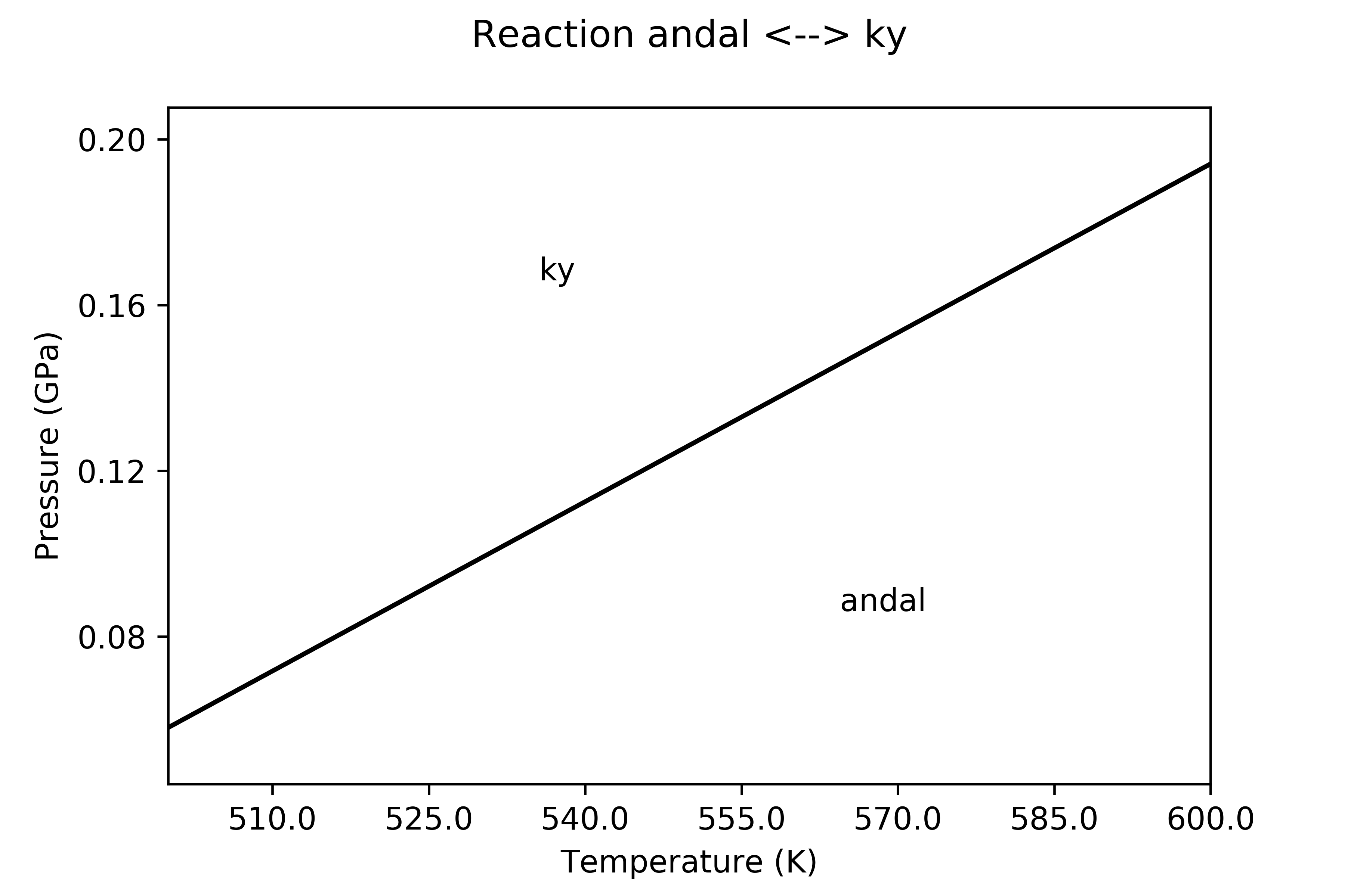
Equilibria between mineral species (only end-members can be considered) can be evaluated starting from the thermodynamic data thus derived. Here is an example where the equilibrium between kyanite and andalusite has been determined in a P/T field: thermodynamics data for kyanite are computed at the QM level, whereas those for andalusite are from literature (Holland & Powell )
All of the properties are computed by constructing the Helmholtz free energy [F(V,T)] as a function of volume (V) and temperature (T). At any given T, F is fitted in a V range by a 3^order volume-integrated Birch-Murnaghan EoS (V-BM3). Results of the fitting are then used to compute all the possibles properties derivable from F.
The program can be loaded and run in a normal Python console as well as in any other environment like Spyder

Jupyter Notebooks or Jupyter Labs are convenient environments, too.
Other than the local PC, Jupyter Notebooks can also be viewed by using the viewer by inserting the location of the book; see the example here .
Once the notebook has been loaded in nbviewer, by clicking on the Execute on Binder button an image is created on the Binder site and the notebook is executed (though it may require some minutes to build the image and run it on the server).
Information about the input required to run the program can be found in the EoS tutorial , as well as in the sections Input file and required files on this site.
The github repository of the package can be found here .
The input files used in the EoS tutorial refer to the example on pyrope and can be found on Github . The notebook of such tutorial can also be view here , on the nbviewer site and, from there, compiled and interactively used on Binder (click on the Execute on Binder icon).
Input description
Download